Simple Linear Regression Model

Fri 13 November 2020

Simple Linear regression assumes that the relationship between a dependent variable y and explanatory variable x, can be modelled as a straight line of the form y = a + b * x; a and b are the regression coefficients. a represents the y‑intercept (the point where a graph of a function intersects the y‑axis), and b the slope (the ratio of vertical change between two points).

Regression is an example of supervised machine learning because it aims to model the relationship between a number of features and a continuous target variable. In the case of simple linear regression, where we aim to model a relationship according y = a + b * x; x would be our feature vector, and y our target variable.

Lets consider the following dataset:

import numpy as np

x = np.arange(0, 11) # 0, 1, .. 10
y = [1, 6, 17, 34, 57, 86, 122, 160, 207, 260, 323]

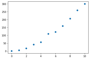
We would like to predict the value of y. Lets plot the dataset to see if we can find some relation between y and x.

import matplotlib.pyplot as plt

plt.plot(x, y, 'o')

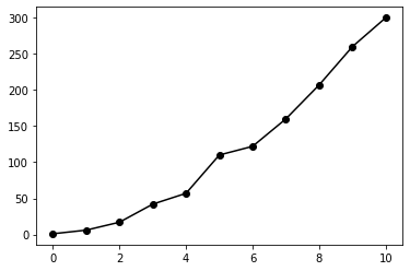
When looking at the dots, in our mind we're likely already visualizing a line which follows a linear path throught the dots. Lets plot again, but now we will include a line which connects the dots.

plt.plot(x, y, '-ok')

Not perfectly linear, but we could probably estimate that y is around 330 at x = 12.

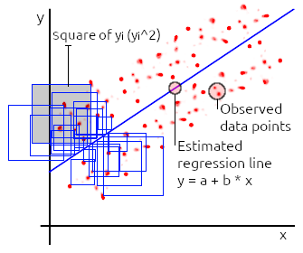
When implementing a linear regression model, we are modelling towards y = a + b * x; in which we aim to estimate the regression coefficients a and b, for a "best fit" of our dataset. To estimate these values we will use sklearn.linear_model.LinearRegression which applies an Ordinary Least Squares (OLS) regression algorithm. This algorithm applies a criteria which aims to minimize the Residual Sum of Squares (RSS). RSS is the sum of squared differences, between the observed y value, and the predicted y value.

Now that we have an idea of what goes on under the hood in sklearn, lets go ahead and implement the code of our linear regression model.

from sklearn.linear_model import LinearRegression

# Data preperation. Convert to numpy arrays, x must be 2-dimensional.
x = np.array(x).reshape((-1, 1))
y = np.array(y)

# Create a model and fit it.
model = LinearRegression()
model.fit(x, y)

print(model.coef_)
# >> 30.745
print(model.intercept_)
# >> -37.182

At this point we have a model available which we can use to make predictions. Note that print statements; print(model.coef_); outputs b, print(model.intercept_); outputs a of y = a + b * x. Lets see what we get when we try to predict y for x = 12.

print(model.predict(np.array([[12]])))
# > array([331.76363636])

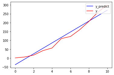
We have a predicted value of y = 331 for x = 12. This looks reasonable, lets print the predicted and observed data in one graph.

y_predict = model.predict(x)

plt.plot(x, y_predict, '-b', label='y_predict')
plt.plot(x, y, '-r', label='y')
plt.legend(loc='upper right')

We can see our prediction is off sometimes. Lets asses the quality of our model by computing the Mean Squared Error (MSE). With MSE we measure the average squared difference between the predicted and observed values. MSE can be computed by mse = 1/n * sum(squared_errors), at which squared_errors is a list of (y_observed - y_predict)**2 entries. MSE is non negative, values close to zero are better (i.e. indicate less error in the predicted versus the observed values). We will use sklearn.metrics.mean_squared_error which makes it very easy to compute the MSE.

from sklearn.metrics import mean_squared_error
print(mean_squared_error(y, y_predict))
# >> 452.691

452.691 is nowhere close to zero, and given that our observed y values are in the 0..300 range, this MSE value basically indicates that this is not a good model for fitting our data. Of course this is not completely surprising, even though we can see some linearity in the graphs, we actually had only 11 datapoints, the model is able to average through these points, but to actually have a good fitting model, we would need a larger amount of data that shows a good amount of linearity in order to apply a linear regression model succesfully.

Category: Modelling